Accordian Closable

7 Tips for Choosing the Best Ultrasonic Disperser?

Choosing an Ultrasonic Disperser is not simply a wattage contest. The right system must suit your sample, target particle size, batch volume, and working routine. A power rating can look reassuring, but it cannot predict dispersion quality by itself. Viscosity, probe diameter, amplitude, vessel shape, and cooling all affect results. Small details matter. A narrow beaker may heat quickly, and a probe placed too close to its wall can produce uneven treatment.

Sonochemistry researcher Kenneth S. Suslick describes ultrasound’s chemical effects as arising from “acoustic cavitation.” That principle helps explain why operating conditions matter: collapsing bubbles transfer energy into the liquid, but the result depends on how the system is configured and used. For a fair comparison, look beyond advertised power. Check whether the unit offers adjustable amplitude, suitable probes, temperature monitoring, and clear guidance for your sample volume. Ask suppliers how their recommendations were tested. Bench results do not always transfer neatly to larger batches.

This guide presents seven practical checks for comparing machines, from sample compatibility and processing capacity to cleaning, controls, and after-sales support. It also flags a common mistake: choosing a unit from a specification sheet without testing the actual material. If possible, run a small trial and record temperature, processing time, and visible changes. Not every sample behaves as expected. That is worth admitting. A careful choice starts with evidence from your own process, not a promise on a product page.

7 Tips for Choosing the Best Ultrasonic Disperser?

Define the Target: Particle Size, Solids Loading, and Viscosity

7 Tips for Choosing the Best Ultrasonic Disperser?
Define the Target: Particle Size, Solids Loading, and Viscosity

Set a measurable particle-size target before comparing equipment. Specify both D50 and D90: the median alone can hide a stubborn coarse fraction. ISO 13320:2020 highlights the importance of documenting dispersion conditions when reporting laser-diffraction results. A finer reading after heavy dilution may not represent the production slurry. Check the sample at its intended concentration, too.

Solids loading changes how particles collide and how ultrasound travels through the batch. Higher loading can increase energy demand and encourage re-agglomeration; viscosity can also dampen cavitation and slow circulation. Record solids percentage, temperature, and viscosity at the process temperature. Small details matter. NIST’s SRM 1963a is a nominal 100 nm polystyrene-particle size reference, useful for checking sizing instruments—not proof that a concentrated slurry is fully dispersed.

Ask suppliers to test your actual formulation across realistic loading and viscosity ranges. Compare the full size distribution, temperature rise, and repeatability, not just one best-case result. A practical trial might reveal that the target size is reached only after excessive heating or long processing. That is worth questioning. Ultrasonic settings are not universal; the right choice depends on the sample, vessel, and scale-up conditions.

7 Tips for Choosing the Best Ultrasonic Disperser

Define the Target: Particle Size, Solids Loading, and Viscosity

Viscosity values illustrate how widely liquid resistance to flow can differ: water is about 1.002 mPa·s, ethanol about 1.20 mPa·s, and glycerol about 1,412 mPa·s at 20°C. Higher viscosity can limit circulation and energy transfer, so evaluate it alongside the required particle size and solids loading when defining your process target. Values vary with temperature, purity, and formulation; these references do not predict disperser performance.

Compare Common Frequencies: 20 kHz Probe Systems vs. 40 kHz Baths

A 20 kHz probe and a 40 kHz bath deliver energy differently. A probe concentrates vibration at its tip, making it useful for breaking stubborn agglomerates in a beaker. A bath spreads sound through the tank, which can suit several small vessels or delicate samples. Chemat and colleagues’ review in Ultrasonics Sonochemistry (2011) describes power ultrasound as commonly operating from 20 to 100 kHz. Both frequencies fall within that range, but frequency alone cannot predict dispersion quality.

The difference is practical. Lower-frequency systems often produce more forceful cavitation, while a 40 kHz bath may provide gentler, broader treatment. Yet vessel shape, sample volume, viscosity, and delivered power can change the result. Suslick’s Science review (1990) reports that cavitation hot spots can briefly reach about 5,000 K and 1,000 atmospheres; these are microscopic, transient conditions, not the bulk sample temperature or pressure. Do not read those figures as a guarantee of performance.

For a probe, watch for a narrow plume, splashing, and local heating. For a bath, check whether the vessel sits in an active zone and whether the liquid level is consistent. I would not choose by frequency alone. That shortcut is tempting, but incomplete. Test a small batch and record treatment time, temperature, and particle-size change.

Size Output by Sample Volume and Delivered Energy in J/mL

7 Tips for Choosing the Best Ultrasonic Disperser?

The right disperser should match both your sample volume and the energy each milliliter needs. A high wattage rating alone does not guarantee effective dispersion. Consider the actual energy delivered to the sample, not just the instrument’s rated power. These are different figures.

Estimate energy density by dividing delivered energy in joules by sample volume in milliliters.

For example, 20,000 joules delivered to 100 milliliters equals 200 J/mL.

Treat this as a starting point, not a universal target. Formulation, viscosity, solids content, probe immersion, and vessel shape all affect how energy is distributed. A thick slurry may respond differently from a thin liquid at the same J/mL.

Choose a unit that can reach your working range without being pushed continuously to its limit. Check whether its controls let you adjust amplitude and processing time, and whether the probe suits your vessel and batch size. Monitor temperature, too; energy can heat a sample quickly, so cooling or pulsed operation may be necessary. Scale-up is rarely neat. Two batches with the same volume can behave differently, and energy estimates may not capture every loss. Record the settings and observed results for each formulation; those notes make the next run more dependable.

Check Probe Materials, Amplitude, and Heat Control for Your Process

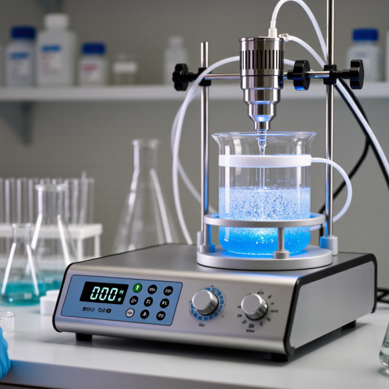
Probe material matters when the tip sits in a corrosive, abrasive, or high-purity mixture. Titanium alloy is common, but it is not automatically compatible with every formulation; check chemical compatibility and wear limits. Amplitude sets the probe’s vibration, not a guaranteed particle size. Start conservatively, then inspect dispersion and the probe tip for wear. Small trials reveal more than guesswork.

Tip: Match the probe diameter to the vessel and batch volume. Keep the tip submerged without letting it touch the vessel wall. Record amplitude, pulse duration, and temperature so a successful run can be repeated.

Heat control is easy to underestimate. Sonication can warm a small sample quickly, changing viscosity or damaging temperature-sensitive ingredients. Use short pulses, a cooling bath, or a jacketed vessel, and measure the liquid temperature—not just the bath. Suslick’s peer-reviewed 1990 Science review describes cavitation bubbles reaching about 5,000 K and 1,000 atmospheres locally; those extreme conditions occur at bubble collapse, not throughout the sample. Still, bulk heating needs monitoring. I would not trust a preset setting alone. A thermocouple near the working zone can expose temperature spikes that a distant display misses.

Verify Particle-Size Results with D10, D50, and D90 per ISO 13320:2020

A disperser’s power rating cannot prove that it produced a stable particle-size distribution. Compare laser-diffraction results before and after treatment under the same sampling and measurement conditions. ISO 13320:2020 describes laser diffraction analysis and reporting; D10, D50, and D90 mark the sizes below which 10%, 50%, and 90% of measured particle volume fall. For example, a report showing D10 = 2 µm, D50 = 8 µm, and D90 = 25 µm indicates a broad distribution, not one “average” particle size. Example values only.

Tips: Ask for repeat measurements and the full percentile distribution, not just D50. Check that the test uses a suitable optical model and consistent sample concentration. NIST reference-material certificates provide certified particle-size values and uncertainty; use an appropriate reference material to check measurement performance near your working range. Keep the sample preparation notes, too. Small differences in dilution or settling can shift the result.

A falling D90 after sonication may indicate fewer large particles, but it does not prove that the dispersion will remain stable. Recheck after a defined resting period. I would also record temperature and treatment time; these details are easy to overlook. One limitation: laser diffraction reports an inferred distribution, so unusual particle shapes or optical properties can complicate interpretation. Compare like with like, then investigate results that do not repeat.

7 Tips for Choosing the Best Ultrasonic Disperser? - Verify Particle-Size Results with D10, D50, and D90 per ISO 13320:2020

Tip What to evaluate Useful data to record How to verify particle-size results
1. Match the disperser to the sample Consider sample volume, viscosity, solids loading, and whether the material is handled as a liquid suspension or dry powder. Confirm that the disperser and vessel can process the required sample volume. Sample volume (mL); solids concentration (% w/w); liquid viscosity (mPa·s); vessel dimensions (mm). Use a representative sample and keep its preparation consistent. Report the sample and dispersion conditions with the particle-size results.
2. Check the operating range Compare the instrument’s rated frequency and power with the application. Nominal power alone does not establish the acoustic energy delivered to the sample; vessel geometry, probe position, and sample properties also matter. Rated frequency (kHz); rated power (W); operating amplitude (%); treatment time (s); pulse settings, if used. Record the settings for each measurement. Evaluate whether D10, D50, and D90 reach a stable result as the treatment conditions are adjusted.
3. Choose suitable probe and vessel geometry Select a probe compatible with the sample volume and vessel. Provide clearance from vessel walls and the bottom, and use a repeatable probe position to reduce variation between runs. Probe-tip diameter (mm); immersion depth (mm); probe-to-wall clearance (mm); vessel material and dimensions. Keep geometry and positioning unchanged between replicates. Compare the particle-size distributions, not just a single median value.
4. Manage heating and sample stability Ultrasonic treatment can heat a sample. Check whether temperature changes, evaporation, or chemical instability could affect the material or the measurement. Initial and final temperature (°C); treatment duration (s); cooling method; visible changes, if any. Use a controlled temperature procedure where needed. Confirm that additional treatment does not cause a continuing shift in D10, D50, or D90.
5. Define a reproducible dispersion procedure Establish a consistent sequence for sample addition, wetting, mixing, ultrasonic treatment, and transfer. Select a compatible dispersing liquid and any additives based on the sample’s chemistry. Dispersant composition; sample mass (g) or volume (mL); mixing time (s); treatment time (s); replicates (n). Document the preparation procedure and repeat measurements under the same conditions. Do not treat one set of settings as suitable for every material.
6. Check for over-dispersion or particle damage More ultrasonic energy is not always better. Excessive treatment may break fragile particles or alter agglomerates that are relevant to the intended application. Treatment time (s); amplitude (%); temperature (°C); changes in distribution with treatment. Run a treatment-time check. A stable distribution can indicate adequate dispersion, while a continuing decrease in size may warrant investigation for particle breakage.
7. Verify results using laser diffraction principles For measurements made by laser diffraction, follow the instrument method and applicable requirements of ISO 13320:2020. The standard describes measurement principles and procedures; it does not prescribe a universal particle-size target for every material. D10, D50, and D90 (µm); distribution basis; optical model and refractive-index inputs; obscuration or concentration setting; replicate results. D10, D50, and D90 are the particle diameters below which 10%, 50%, and 90% of the reported cumulative distribution fall, respectively. State the distribution basis and measurement conditions when reporting them.

Reporting note: D10, D50, and D90 values depend on the sample preparation and measurement conditions. Compare results only when the dispersion procedure, instrument method, and distribution basis are suitably consistent.

Article Source: